Week 2
| Class | C4W2 |
|---|---|
| Created | |
| Materials | |
| Property | |
| Reviewed | |
| Type |
Case Studies
Classic Networks
In this section we will look at some of the classic neural networks architectures, namely:
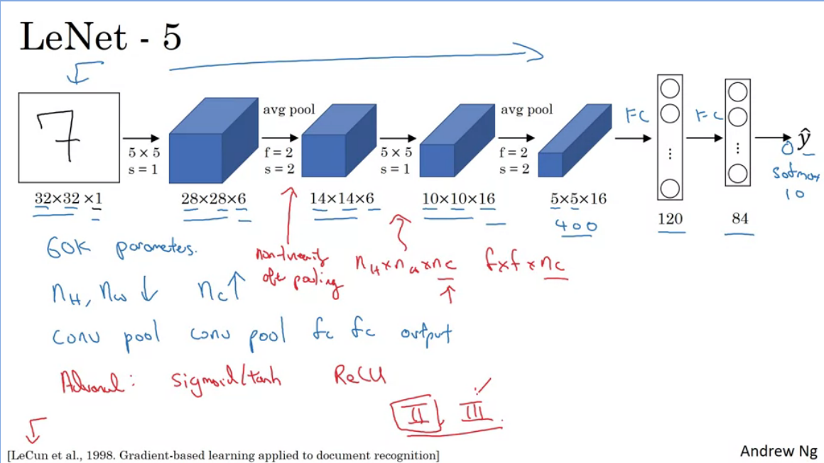
The main goal of LeNet-5 was to recognise hand written digits.
- 60 000 parameters
- nH and nW tend to descrease while nC increases
- The common arrangement of layers is common as it follows the standard of: Conv→Pool→Conv→Pool→FC→FC→Output
It turns out if you read the paper, that people used sigmoid and tanh non-linearities instead of ReLu, and had non-linearities after pooling.
Useful resource: https://towardsdatascience.com/review-of-lenet-5-how-to-design-the-architecture-of-cnn-8ee92ff760ac
AlexNet
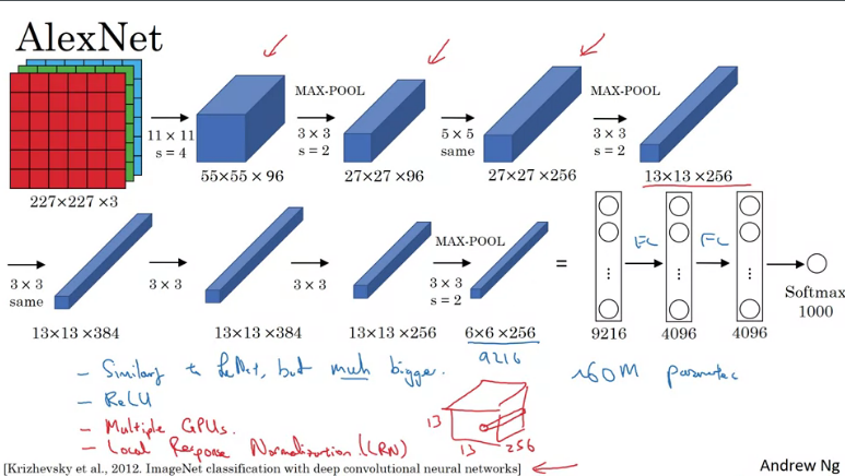
This network had a lot of similarities to LeNet-5, but this had over 60million parameters, when training a lot of the layers where trained on multiple GPU's.
VGG-16
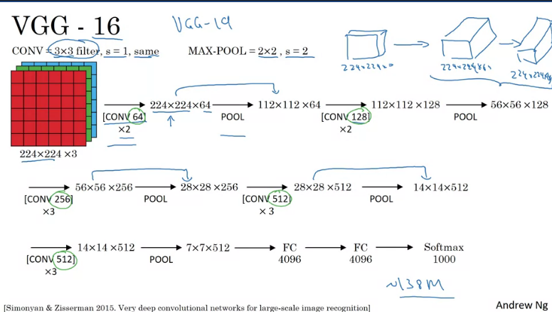
One of the remarkable things with VGG-16 net is that instead of having many hyperparameters it was actually simplified to just a few hyperparameters, Conv-layers that are 3x3 filters with a stride of 1 and always use same adding, all max pooling layers are 2x2 with a stride of 2. The 16 in VGG refers to the number of layers that have weights. This is a large network with a total of 138 million parameters.
ResNets
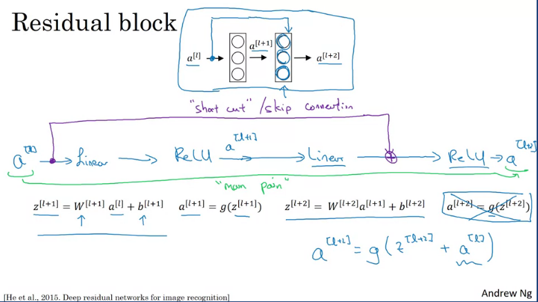
Very, very deep neural networks are difficult to train because of vanishing and exploding gradient types of problems. In this section, we will learn about skip connections which allows you to take the activation from one layer and suddenly feed it to another layer even much deeper in the neural network. And using that, we'll build ResNet which enables you to train very, very deep networks. Sometimes even networks of over 100 layers.
ResNets are built out of something called residual blocks.
What the authors found was that using residual blocks allows you to train much deeper neural networks and the way to build is by taking many of these residual blocks and stacking them together to form a deep network.
To turn a "plain network" into a residual network you would need to skip networks as show in the image(blue lines).
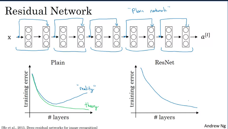
In theory having a deeper network should help with the training, however, in practice havin a plain network which is deep simply means that all your optimization algorithm just has a much harder time training and training error gets worse.
But with ResNets, even as the number of layers gets deeper, the perfomance of the training error continously goes down, even if trained with over a hundred layer.
Resource: https://d2l.ai/chapter_convolutional-modern/resnet.html#
Why ResNets Work?
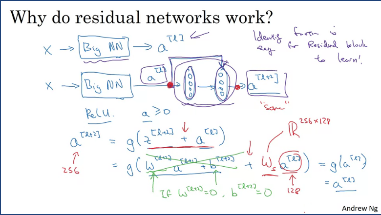
Suppose you have an input X which feeds into a big nn and the output is and want to modify it such that it becomes a ResNet to make it a little deeper by adding few layers to the network. By adding 2 layers and making them residual blocks with a skip connection, the output of the network will thus be (assuming we using the ReLu activation) which equates to and if using weight decay this will mean that then .
This shows that the identify function is easy for the residual block to learn. This is why adding a residual block into our network does not hurt the perfomance, and gradient descent can thus increase perfomance (might).
How ResNet work on images
This image shows an example of a plain network which takes in an input image and then have a number of conv-layers until eventually a softmax on the output.

In order to turn this network into a ResNet we would need to skip connections. Note that theres a number of similar 3x3 convolutions and most of them have 3x3 convolutions so the dimensions are preserved and there's occasional pooling layers and the end you have fully connected layer which then makes a prediction using a softmax.
Networks in Networks and 1x1 Convolutions
In terms of designing convnet architectures, one of the ideas that really helps is using a one by one convolution. Now, you might be wondering, what does a one by one convolution do? Isn't that just multiplying by numbers? That seems like a funny thing to do. Turns out it's not quite like that.
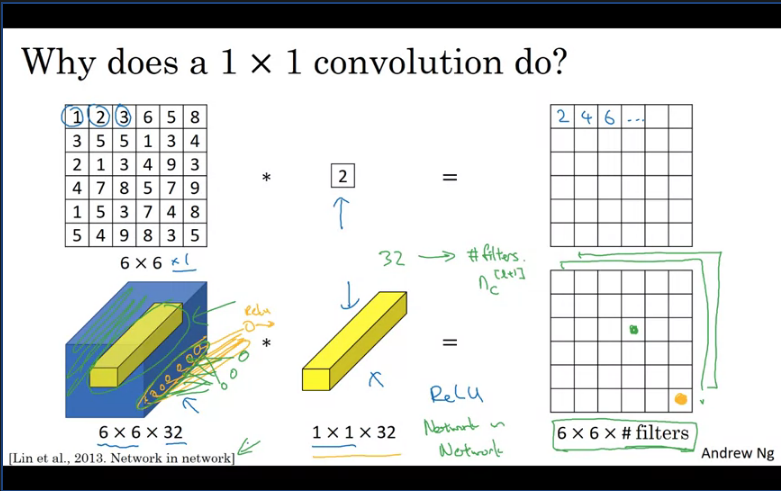
Consider a 1x1 filter with a value of 2 and convolve it with an input image the product will just be doubled values of the input image which doesn't really seem particulary useful. However, if you have a input with more channels and convolve it with a 1 x 1 x n_C filter then the output will thus contain n_C number of filters.
One way of thinking about the n_C numbers you have in the filter is that, it's as if you have a neuron that is taking an input number and multiplying each of the numbers in one slice of the same position height and width of the numbers in one slice of the same position n_H and n_W by these different channels then multiplying them by weights and then applying ReLU non-linearity to it before the output.
Usage
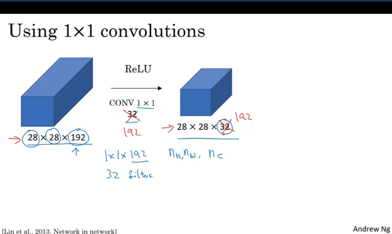
Suppose have an input and you want to shrink only the n_C and not the n_H and n_W of which n_H and n_W can be shruken using a pooling layer.
You could use a 32 1x1 filters with the same n_C as the input this would output n_H, n_W, n_C= # of filters.
This 1x1 convnet allows you to shrink or increas the number of channels in your volume which is useful to the inception network.
Inception Network Motivation
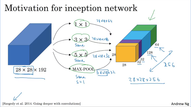
Suppose we have an input of 28x28x192 dimensional volume, what the inception network or inception layer does is instead of choosing what filter size you want in your Conv layer or if you want a Conv or pooling layer - let's do them all.
With the inception module you can input some volume and output then add yo all those number (32+32+128+64 = 256). So you will have one inception module input 28x28x192 outputting a 28x28x256 volume.
Inception Network/GoogleNet
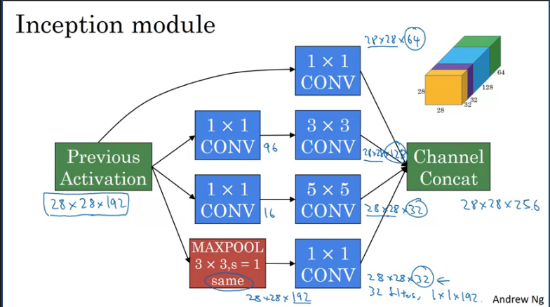
The inception module takes as input the activation or the output from some previous layer. In our case this is a 28x28x192 which goes through a 1x1x16 conv then 5x5 conv then the output will be 28x28x32. The do the same for the 1x1x96 and 3x3 convolution, the output will be 28x28x128. The consider a 1x1 convolution which will output 28x28x64
In order to really concatenate all of these outputs at the end we use the same type of padding for pooling. So that the output height and width stays as 28x28. But notice that if you do max-pooling, even with same padding, 3x3 filter is tried at 1. The output here will be 28x28x192. It will have the same number of channels and the same depth as the input that we had here. This seems like is has a lot of channels. So what we're going to do is actually add one more 1x1 conv layer to strengthen the number of channels. So it gets us down to 28x28x32. And the way you do that, is to use 32 filters, of dimension 1x1x192. So that's why the output dimension has a number of channels shrunk down to 32. So then we don't end up with the pulling layer taking up all the channels in the final output.
Finally you take all of these blocks and you do channel concatenation. Just concatenate across this 64x128x32x32 and this if you add it up this gives you a 28x28x256 dimension output.
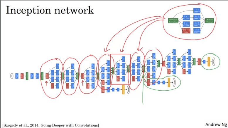
if you understand the inception module, then you understand the inception network. Which is largely the inception module repeated a bunch of times throughout the network. Since the development of the original inception module, the author and others have built on it and come up with other versions as well. So there are research papers on newer versions of the inception algorithm.
Practical advices for using ConvNets
Transfer Learning
Suppose you are building a computer vision application instead of training your algorithm from scratch (random initialization), you would often progress faster if you leverage the use of already trained network architectures by using that as pre-training and transfer that to a new task that you might be interested in.
The computer vision research community has vast number of open source data sets such as ImageNet, or MS COCO, or Pascal types of data sets, these are the names of different data sets that people have post online and a lot of computer researchers have trained their algorithms on. Sometimes these training takes several weeks and might take many GPU and the fact that someone else has done this and gone through the painful high-performance search process, means that you can often download open source ways that took someone else many weeks or months to figure out and use that as a very good initialization for your own neural network. And use transfer learning to sort of transfer knowledge from some of these very large public data sets to your own problem.
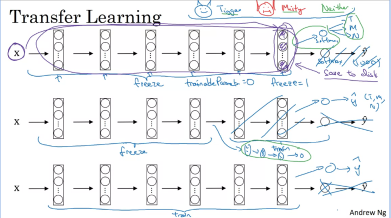
Suppose you want to create a cat classifier application using transfer learning, there are 3 options in order to achieve that, you would need to initially download an already pre-trained model (that was trained on multiple classes) and;
- Freeze the parameters on all layers and only train the parameters associated with your output softmax layer, which will be your classification layer.
- This assumes you have a small dataset.
- Freeze fewer layers and only train the last few layers (1. You could take the last few layers and use that as initialization then do gradient descent, or 2. Remove last few layers and use your own new hidden layers then a final softmax classifier).
- This assumes you have a large dataset
- Unfreeze and train the whole network and only replace the softmax output classifier, which might take a long time depending on your computational resources.
- This assumes you have a very large dataset
In practice, when working with transfer learning most researchers opt for option 1 or 2 as it doesn't require a lot of computational resources and already the heavy lifting has been done for them.
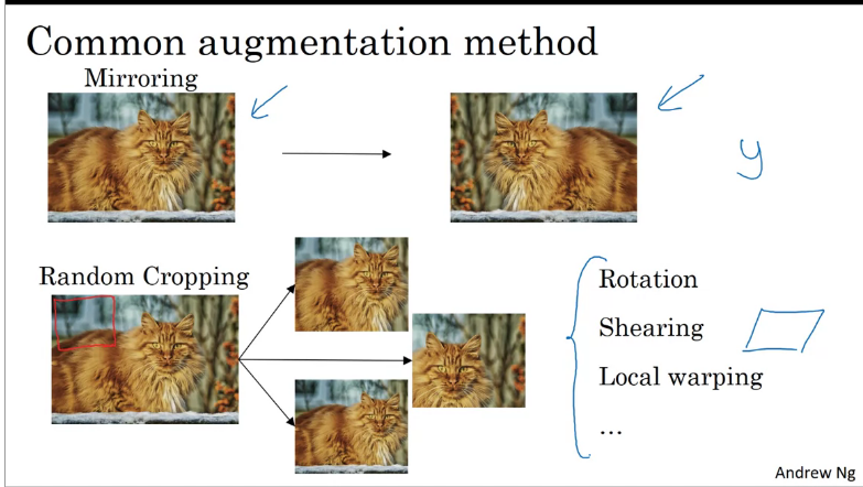
Data Augmentation
Often, when you're training computer vision models, data augmentation helps especially when you have a small dataset.
According to https://developers.google.com/machine-learning/glossary#data-augmentation, It can be defined as artificially boosting the range and number of training examples by transforming existing examples to create additional examples.
For example, suppose images are one of your features, but your dataset doesn't contain enough image examples for the model to learn useful associations. Ideally, you'd add enough labeled images to your dataset to enable your model to train properly. If that's not possible, data augmentation can rotate, stretch, and reflect each image to produce many variants of the original picture, possibly yielding enough labeled data to enable excellent training.
Common data augmentation methods used in computer vision.
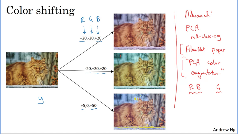
Another advanced method used is color shifting.
How is data augmentation implemented during training
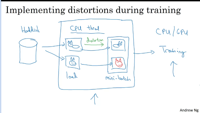
Suppose you have some data input, you would need to add a function that would distort (note this is parameterised) your images before training, ideally on a separate thread.
State of Computer Vision
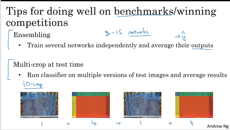
Tips for doing well on benchmarks/winning competitions
Use open source code
- Use architectures of networks published in the literature.
- Use open-source implementations if possible.
- Use pretrained models and fine-tune on your dataset.
Q & A
Deep convolutional models
- Which of the following do you typically see as you move to deeper layers in a ConvNet?
- nH and nW decrease, while nC increases
- Which of the following do you typically see in a ConvNet? (Check all that apply.)
- Multiple CONV layers followed by a POOL layer
- FC layers in the last few layers
- In order to be able to build very deep networks, we usually only use pooling layers to downsize the height/width of the activation volumes while convolutions are used with “valid” padding. Otherwise, we would downsize the input of the model too quickly.
- False
- Training a deeper network (for example, adding additional layers to the network) allows the network to fit more complex functions and thus almost always results in lower training error. For this question, assume we’re referring to “plain” networks.
- False
- The following equation captures the computation in a ResNet block. What goes into the two blanks above?
- a[l] and 0, respectively
- Which ones of the following statements on Residual Networks are true? (Check all that apply.)
- Using a skip-connection helps the gradient to backpropagate and thus helps you to train deeper networks
- The skip-connections compute a complex non-linear function of the input to pass to a deeper layer in the network.
- Suppose you have an input volume of dimension 64x64x16. How many parameters would a single 1x1 convolutional filter have (including the bias)?
- 17
- Suppose you have an input volume of dimension nH x nW x nC. Which of the following statements you agree with? (Assume that “1x1 convolutional layer” below always uses a stride of 1 and no padding.)
- You can use a 1x1 convolutional layer to reduce nC but not nH, nW.
- You can use a pooling layer to reduce nH, nW, and nC.
- Which ones of the following statements on Inception Networks are true? (Check all that apply.)
- A single inception block allows the network to use a combination of 1x1, 3x3, 5x5 convolutions and pooling.
- Inception blocks usually use 1x1 convolutions to reduce the input data volume’s size before applying 3x3 and 5x5 convolutions.
- Which of the following are common reasons for using open-source implementations of ConvNets (both the model and/or weights)? Check all that apply.
- It is a convenient way to get working an implementation of a complex ConvNet architecture.
- Parameters trained for one computer vision task are often useful as pretraining for other computer vision tasks.