Week 2
| Class | C2W2 |
|---|---|
| Created | |
| Materials | https://www.coursera.org/learn/deep-neural-network/home/week/2 |
| Property | |
| Reviewed | |
| Type | Section |
Algorithm Optimization techniques
Mini-batch gradient descent
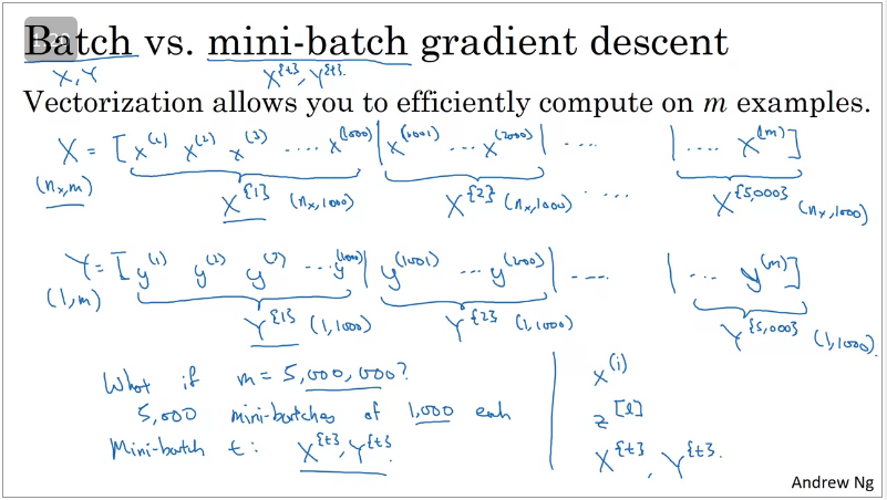
Suppose , this can not be computed easily using ordinary batch gradient descent (very large dataset) using vectorization which allows you to process all exaples of
It turns out, that there's an algorithm which helps you to process large datasets which is mini-batch gradient descent. This type of gradient descent, splits the training data into small batches that are used to calculate model errors and update model coefficients one batch after the other. Thus optimising your algorithms perfomance and decreasing training time.
Understanding mini-batch gradient descent
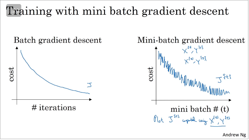
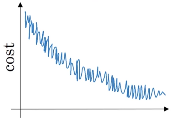
- Batch gradient descent - With every iteration you go through the entire training set and should expect the cost function to decrease with every iteration., whereas with
- Mini-batch gradient descent - With every iteration you processing a value of and should you plot the cost function you are more likely to see the graph illustrated above which is a lot more noisier, where at every iteration you're training on a different training set or rather a different mini batch which should trend downwards.
Choosing your mini-batch size (Hyperparameter)
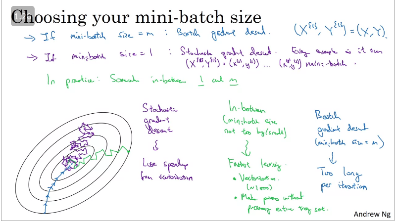
- If your
mini-batch size, then you end up with batch gradient descent (This mini batch equals your whole training set) i.e too long per iteration
- If your
mini-batch sizethen you end up with a stochastic gradient descent.
- If your
mini-batch size =~, Faster learning and vectorization
Stochastic gradient descent
The word 'stochastic' means random process.
- Few samples are randomly selected instead of the whole dataset at each iteration to compute gradient descent, most times you would move towards the global minima or change direction.
- It can be used for larger dataset, it converges faster when the dataset is large as it causes updates to the parameters more frequently.
- Since a random sample is selected at each iteration, this means that if we plot our cost function it will be more noisier than a typical gradient descent algorithm.
- noisiness can be improved by using a smaller learning rate...
- Disadvantage: Loose vectorization speed
See stochastic gradient descent algorithm explained:
Key takeaways when choosing a mini-batch size:
- If you have a small training set (, use batch gradient descent.
- Typically choosing mini-batch size should be
- Ensure that your mini-batch fits into your CPU/GPU memory else perfomance lags.
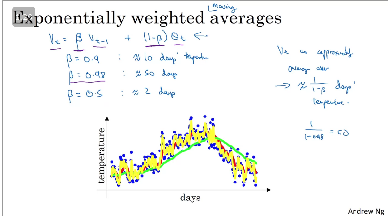
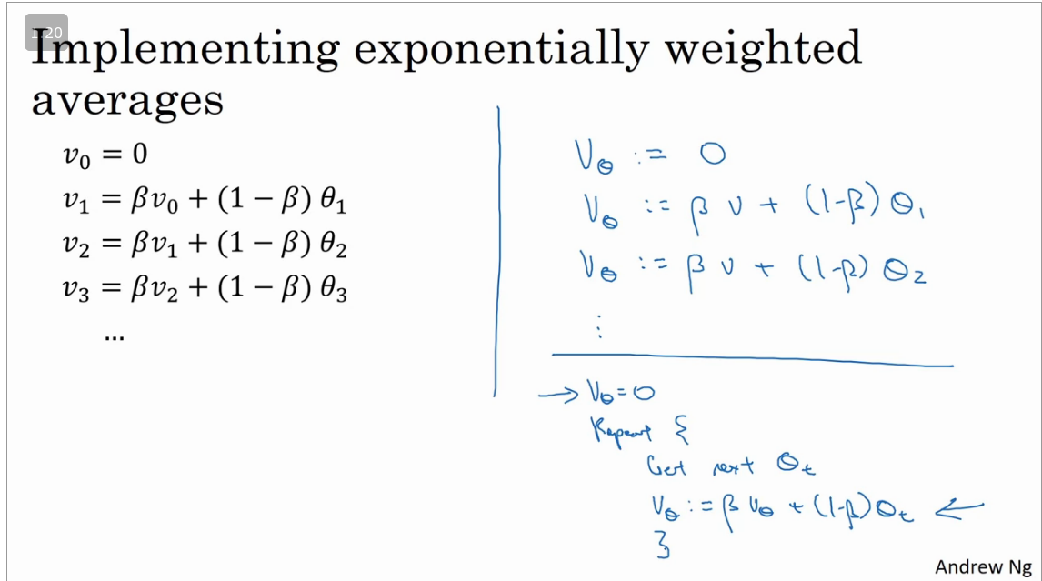
Exponentially weighted (moving) averages
From wikipedia, EWA/EWMA is a first-order infinite impulse response filter that applies weighting factors which decrease exponentially. The weighting for each older datum decreases exponentially, never reaching zero.
Bias correction in exponentially weighted averages
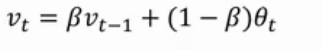
Gradient descent with momentum
This algorithm computes an exponentially weighted average of your gradients, and then use that gradient to update weights instead.
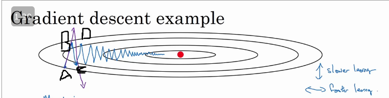
Consider the image above, where we are computing gradient descent without momentum. In this case you are trying to compute cost function , so the red dot in the middle denotes the position of the minima. Suppose at the first iteration the gradient descent moves from 'A' and end up at 'B' which is on the otherside of the ellipse, and take another step of the gradient descent from 'B' and end up at 'C' and so on...
The gradient descent will move towards the minimum after a number of oscillations/steps which slows would slow it down and prevent's us from using a much higher learning rate as with larger learning rate gradient descent might shoot up/down and diverge.
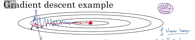
If we compute gradient descent with momentum (viz aviz. moving averages), we would find out that the oscillations in the vertical direction will tend to average out to a value closer to zero and all the derivatives on the horizontal direction will be larger causing a smoother gradient descent.
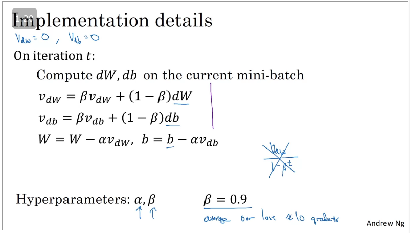
Momentum works because, we don't compute the exact derivative/slope of the cost function , instead we estimate it on small batches.
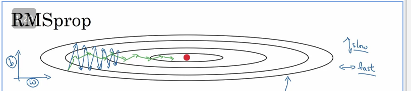
RMSprop
Root Mean Square propagation, The motivation is that the magnitude of gradients can differ for different weights, and can change during learning, making it hard to choose a single global learning rate. RMSProp tackles this by keeping a moving average of the squared gradient and adjusting the weight updates by this magnitude.
The impact of using RMSprop is that the gradient descent is much faster to compute( larger learning rate) and dampens the oscillation due to the squaring of the derivatives and then taking the square root at the end..
Further reading: https://towardsdatascience.com/understanding-rmsprop-faster-neural-network-learning-62e116fcf29a
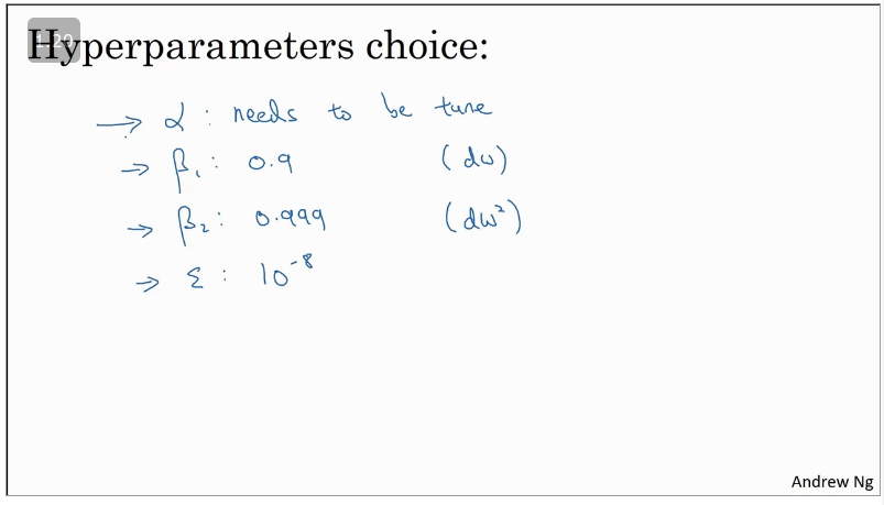
Adam Optimisation algorithm
The Adam(Adaptive Moment Estimation) optimizer basically combines the best properties of the gradient descent with momentum and RMSprop in order to provide an optimisation algorithm than can handle sparse(close to zero) gradients on noisy problems.
Some advantages:
- Low memory requirements
- Works well with minimal turning of hyperparameters.
Paper:
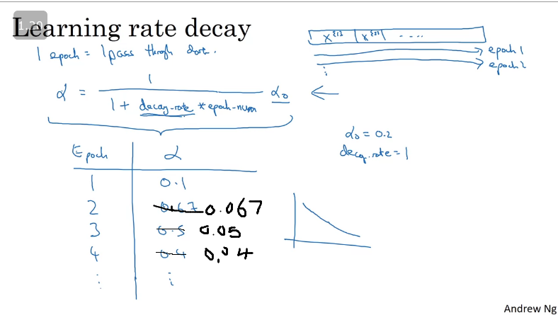
Learning rate decay
One of the things that might increase the speed of your learning algorithm is slowly reducing the learning rate overtime. The intuition behid reducing the learning rate is that during the initial steps of learning, you could take much bigger steps and then as learning approaches converges then having a slower learning rate allows you to take smaller steps.
Learning rate decay implementation:
Useful Resources:
Hinton, 2012: Neural Networks for Machine Learning
Q & A
- Which notation would you use to denote the 3rd layer’s activations when the input is the 7th example from the 8th minibatch?
-
- Which of these statements about mini-batch gradient descent do you agree with?
- One iteration of mini-batch gradient descent (computing on a single mini-batch) is faster than one iteration of batch gradient descent.
- Why is the best mini-batch size usually not 1 and not m, but instead something in-between?
- If the mini-batch size is m, you end up with batch gradient descent, which has to process the whole training set before making progress.
- If the mini-batch size is 1, you lose the benefits of vectorization across examples in the mini-batch
- Suppose your learning algorithm’s cost JJJ, plotted as a function of the number of iterations, looks like this:
Which of the following do you agree with?
- If you’re using mini-batch gradient descent, this looks acceptable. But if you’re using batch gradient descent, something is wrong.
5. Suppose the temperature in Casablanca over the first three days of January are the same:
Jan 1st:
Jan 2nd:
(We used Fahrenheit in lecture, so will use Celsius here in honor of the metric world.)
Say you use an exponentially weighted average with to track the temperature: If is the value computed after day 2 without bias correction, and is the value you compute with bias correction.
What are these values? (You might be able to do this without a calculator, but you don't actually need one. Remember what is bias correction doing.)
-
6. Which of these is NOT a good learning rate decay scheme? Here, t is the epoch number.
-
7. You use an exponentially weighted average on the London temperature dataset. You use the following to track the temperature: . The red line below was computed using . What would happen to your red curve as you vary ? (Check the two that apply)
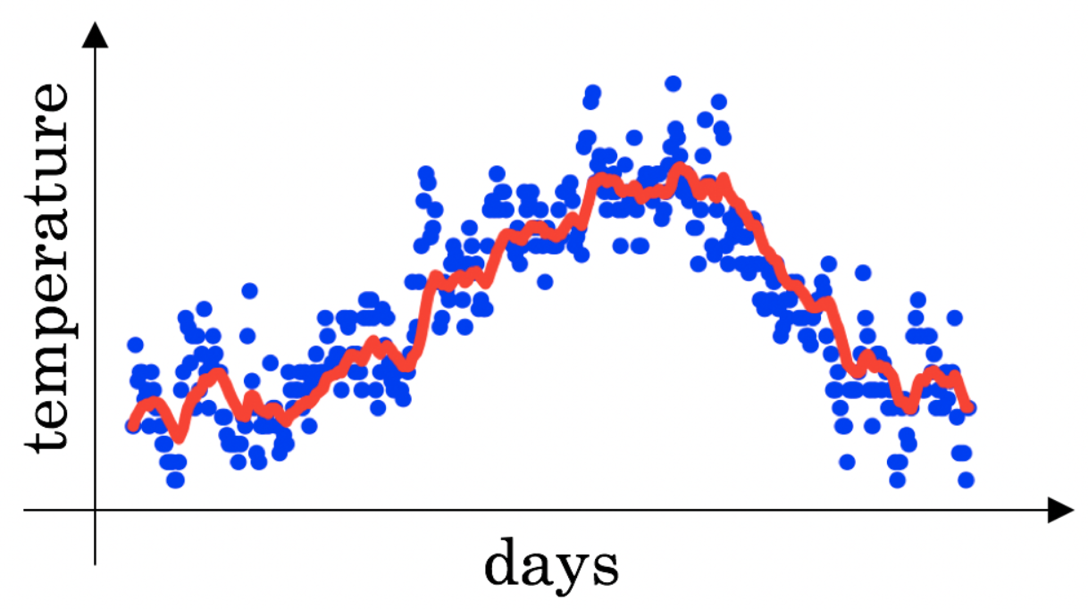
- Increasing will shift the red line slightly to the right.
- Decreasing will create more oscillation within the red line.
8. Consider this figure:
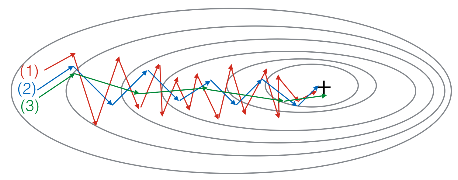
These plots were generated with gradient descent; with gradient descent with momentum and gradient descent with momentum . Which curve corresponds to which algorithm?
- (1) is gradient descent with momentum (). (2) is gradient descent. (3) is gradient descent with momentum ()
9. Suppose batch gradient descent in a deep network is taking excessively long to find a value of the parameters that achieves a small value for the cost function . Which of the following techniques could help find parameter values that attain a small value for? (Check all that apply)
- Try tuning the learning rate
- Try using Adam
- Try mini-batch gradient descent
10. Which of the following statements about Adam is False?
- Adam should be used with batch gradient computations, not with mini-batches.