Week 1
| Class | C2W1 |
|---|---|
| Created | |
| Materials | https://www.coursera.org/learn/deep-neural-network/home/week/1 |
| Property | https://www.coursera.org/learn/neural-networks-deep-learning/ |
| Reviewed | |
| Type | Section |
Setting up your Machine Learning Application
Train / Dev / Test sets
When starting off a machine learning project you need to make a lot of decisions such as:
- The number of layers
- The number of hidden layers each layer should have
- The type of activation for your project
- The learning rate
But this doesn't come easy as ML is a highly interactive process, it takes a while until you find optimised solutions but one of the things that will determine how quickly you make progress is how efficiently you can go around the process cycle.
Setting up your training, cross-validation and test set can go a long way as adjusting your sets could get you highly optimised solution...
→ One thing to note is to make sure that your cross-validation and test set comes from the same distribution as this might influence your end product.
→ It is also okay not to have a test set as long as the cross-validation set is available (as x-validation is technically testing).
Bias / Variance
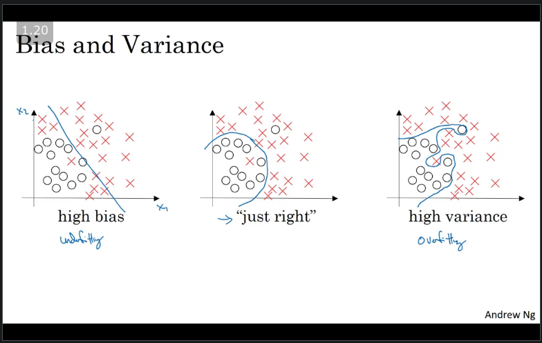
Bias refers to the difference between your model's expected predictions and the true values and, Variance refers to your algorithm's sensitivity to specific sets of training data.
From the image above, imagine fitting a linear/logistic regressing to a dataset that has a non-linear pattern. A linear/logistic regression will not be able to model the curves in the data. This is known as Under-fitting. occurs when there's high bias.
Now with the same data, imagine our algorithm fors completely unconstrained, super-flexible to the same dataset. This is known as Over-fitting occurs when there's high variance.
But there might be a classifier in between with a medium level of complexity that fits correctly we refer to this as Just right which simplly means that theres low bias and low varience.
Ref: https://elitedatascience.com/bias-variance-tradeoff
Key takeaway:
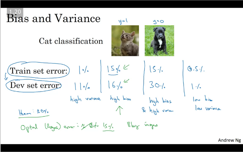
- By looking at the Train set error rate you can get a sense of how well your model is perfoming on the training set and that would tell you if you have a bias problem or not and,
- Looking at how much higher your error goes from training set to cross-validation set, that should give you a sense of how bad is the varience problem.
- However, the error rates are based on human perception of error which is assumed to be 0% error this is also called the Optical/ Bayes error
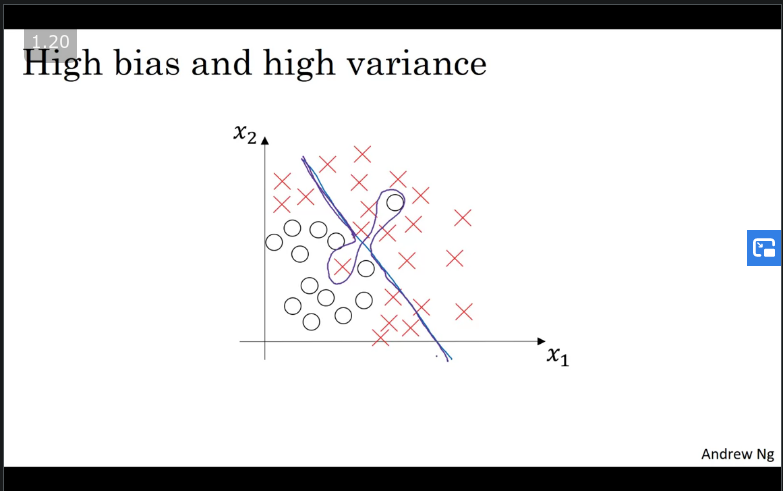
In the case of your model under-fitting and over-fitting at the same time, were it has a high bias by being a linear/logaristic classifier is not fitting and being flexible in the middle this would be an example of overfitting.
Basic recipe for Machine Learning
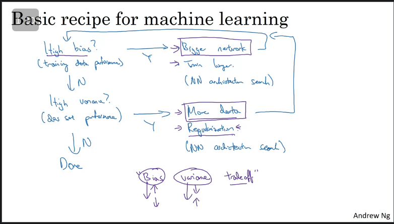
In the previous section we saw how observing our training error and cross-validation error can help diagnose whether our algorithm has a bias or a varience problem or both.
Ways of improving your algorithms perfomance (this is an interative process):
- If initial model has High Bias;
- Look at the training data set perfomance.
- Increase your NN (more layers and more hidden layers)
- Increase time to train.
- Once the Bias has been removed, evaluate whether you have High Variance (if yes);
- Collect more training data
- Regularisation in order to reduce over fitting.
- An alternative NN architecture
Regularizing your neural network
If you suspect that your networks is overfitting your data, you might have a high variable problem, one of the firsth things you should consider is regularization.
From wikipedia, Regularization is the process of adding information in the order to solve or prevent overflitting.
Great explaination with analogies for better understanding: https://developers.google.com/machine-learning/crash-course/regularization-for-simplicity/video-lecture
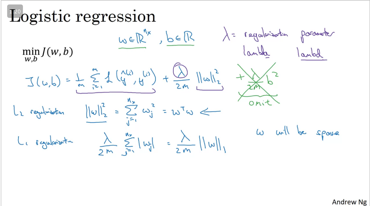
Recall that in logistic regression, you are trying to minimise the cost function . So in order to minimize overfitting on regressiion problems you would need to add the regularization parameter with an efficient reqularization technique (preferably L2 regulatization) - this parameter is part of the hyperparameters and the value depends on the problem.
There are three efficient regularizarion techniques, namely:
- Dropout (See next section)
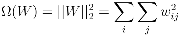
- Euclidian (L2) regularization this is the most common type of regularization which penalizes weights in propotion to the sum of the squares of the weights. It helps drive weight vectors closer to 0 but not quite 0 (as compared to L1) which is also refered to as weight decay
🤖The Best Artificial Intelligence, Machine Learning and Data Science Resources* . And is denoted by the formula below.
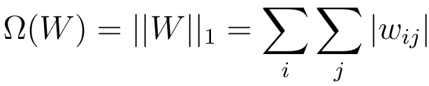
- L1 regularization constrasts with L2 regularization, this type of regularization penalises weights in proportion to the sum of the absolute values of the weights.
- Note: If you use L1 regularization your weights will be sparse i.e some of your weight vectors will comprise of zeros thus compressing your model (save memory) which might only help a little.
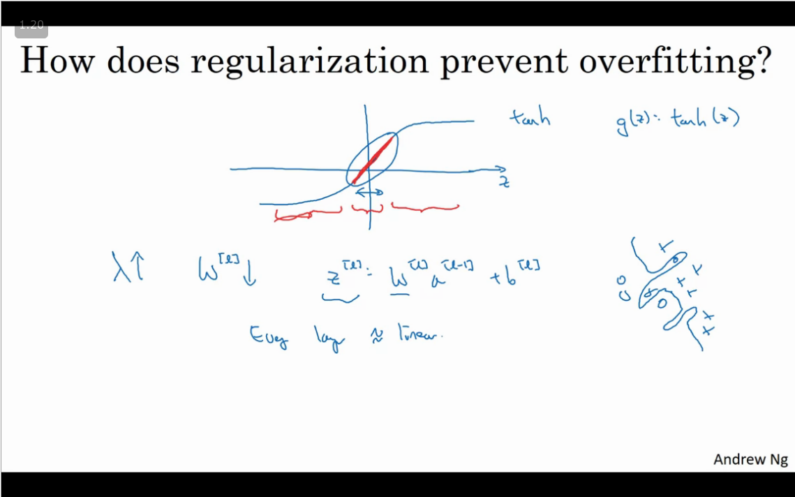
When computing the regularization on a neural network we add lambda over the sum all W parameters and the w parameter matrix which is refered to as squared norm. Where the squared norm is the L2 regularization. Computing gradient descent with L2 regularization is just a mere adding the regularization parameter and matrix norm (highlighted in red)
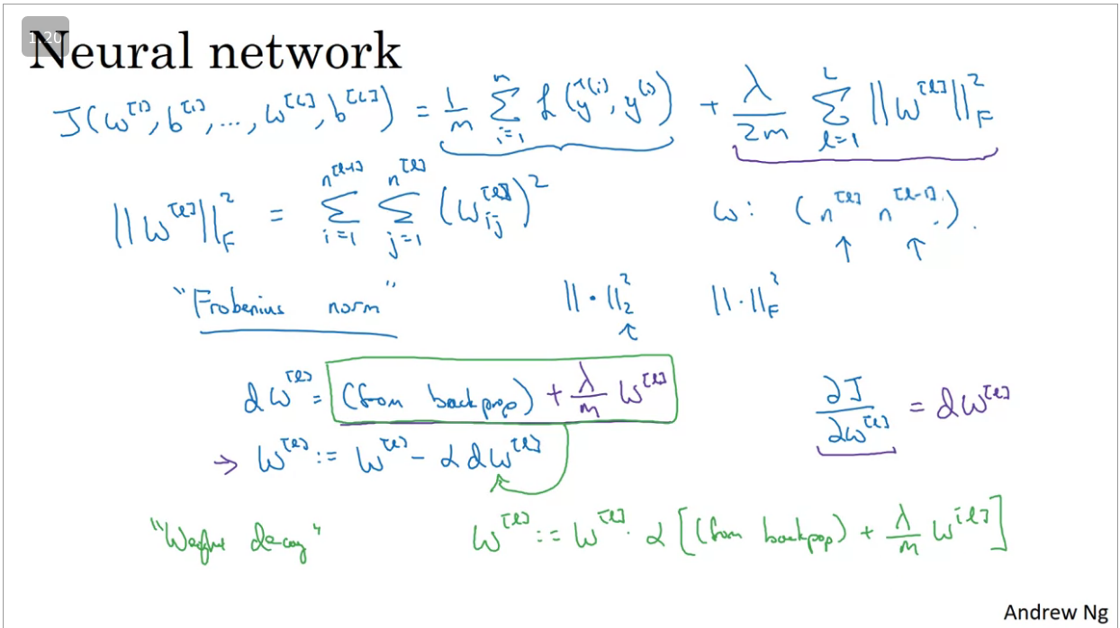
Note: When setting up regularization parameters (), if regularization is large then the weight parameters will be very small thereby affecting the value of Z making it very small. The neural network therefore functions as a very complex linear regression.
What you should remember -- the implications of L2-regularization on:
- The cost computation:
- A regularization term is added to the cost
- The backpropagation function:
- There are extra terms in the gradients with respect to weight matrices
- Weights end up smaller ("weight decay"):
- Weights are pushed to smaller values.
Some useful resources:
Dropout Regularization
This type of regularization, works by removing random selection of fixed number of units in a network layer for a single gradient descent step. See: https://developers.google.com/machine-learning/glossary#dropout-regularization
The downside to dropout regularization is that your cost function J becomes redundant as the networks changes at every gradient descent calculation.
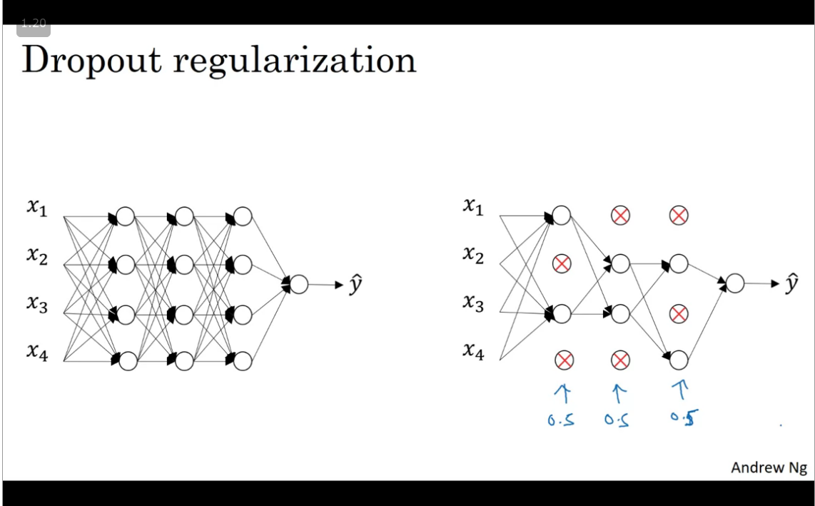
Dropout is a widely used regularization technique that is specific to deep learning. It randomly shuts down some neurons in each iteration. Watch these two videos to see what this means!
When you shut some neurons down, you actually modify your model. The idea behind drop-out is that at each iteration, you train a different model that uses only a subset of your neurons. With dropout, your neurons thus become less sensitive to the activation of one other specific neuron, because that other neuron might be shut down at any time.
- A common mistake when using dropout is to use it both in training and testing. You should use dropout (randomly eliminate nodes) only in training.
- Apply dropout both during forward and backward propagation.
- Deep learning frameworks like tensorflow, PaddlePaddle, keras or caffe come with a dropout layer implementation. Don't stress - you will soon learn some of these frameworks.
See journal paper:
Dropout: A Simple Way to Prevent Neural Networks from Overfitting
Other regularization methods
Data augmentation → https://developers.google.com/machine-learning/glossary#data-augmentation
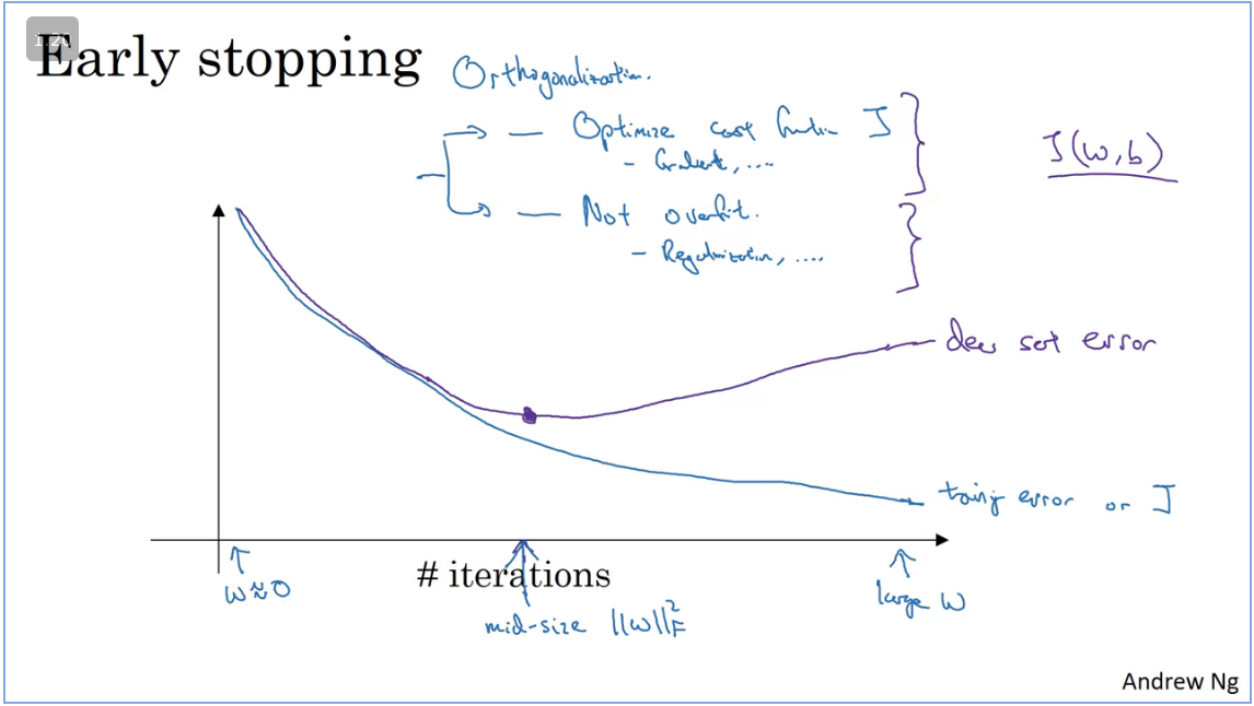
Early stopping → https://developers.google.com/machine-learning/glossary#early-stopping
- Downside for using early stopping, is that when stopping the calculation gradient descent midway this affects the cost function. Alternatively consider using L2 regularization
Setting up your optimization problem
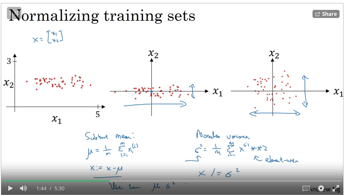
Normalizing Inputs
When training a neural network one of the techniques that will speed up the training time is to normalize your inputs, this means that converting range of values into a standard range of values. Typically ranging from -1 to +1 or 0 to 1
https://developers.google.com/machine-learning/glossary#normalization
Vanishing/Exploding gradients
One of the issues when training neural networks is that of vanishing/exploding gradients which means that during training a deep network your derivatives/slope can get very big or very small thus making training difficult.
Detailed explaination: https://developers.google.com/machine-learning/glossary#vanishing-gradient-problem and https://developers.google.com/machine-learning/glossary#exploding-gradient-problem
Key takeaway:
- if your weight vectors are 1 (identity matrix) then with a deep netwrok the activations can explode.
- However, with weight vectors 1, then the activations will decrease explonentially.
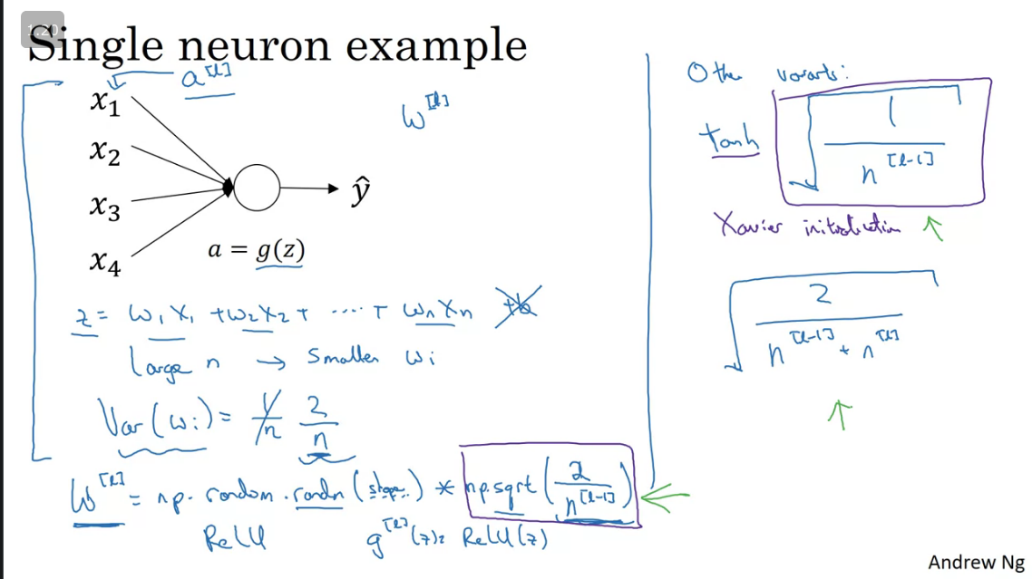
Weight initialization for deep networks
To ensure that your network does not have vanishing/exploding gradient you would need to initialize your weights and multiply them with an initialization vector(hyperparameter).
When your activation function is a ReLU use a multiplier of np.sqrt(2/n^(l-1)) and when using user Xavier initialization
The sole purpose of doing this is just to ensure that the weight vectors are not more than 1 or closer to 0 which will cause vanishing/exploding gradients.
Xavier initialization explained: https://prateekvjoshi.com/2016/03/29/understanding-xavier-initialization-in-deep-neural-networks/
Understanding inititializations techniques and the math behind it: https://towardsdatascience.com/weight-initialization-in-neural-networks-a-journey-from-the-basics-to-kaiming-954fb9b47c79
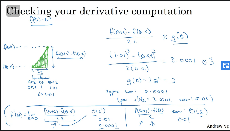
Numerical approximation of gradients
When implementing back propagation there's a test called gredient checking that can ensure that back propagation is correct (See the implemetation on the coding exercize). Inorder to do gradient checking we need to numerically approximate computations of gradients.
You can numerically verify if your function is a correct implemantation of the derivative of a function , ( by using the fomula below:
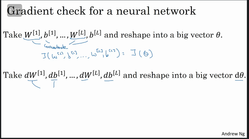
Grad(ient) Checking
Example on implemeting gradient checking: https://towardsdatascience.com/coding-neural-network-gradient-checking-5222544ccc64
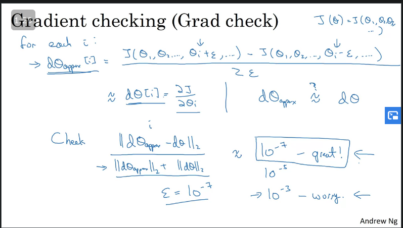
Key takeaway:
- Implemeting gradient checking you would need to compute the euclidien distance between the approximated value and actual value and if it's below your back propagation logic is great else there's a problem.
- Don't use grad checking in training - only when debugging.
- If an algorithm fails grad check, look at components to try to identify a bug.
- Remember regularization ( is gradient of with respect to )
- Doesn't work with dropout. (alt, turn of dropout
keep_prop=1.0compute grad check then turn back on)
- Run at random initialization, perhaps again after some training.
Something to remember:
- Regularization will help you reduce overfitting.
- Regularization will drive your weights to lower values.
- L2 regularization and Dropout are two very effective regularization techniques.
- Normalizing your inputs will speed up your training time.
- Initialize your weights to avoid vanishing/exploding gradients.
Q & A
- If you have 10,000,000 examples, how would you split the train/dev/test set?
- 98% train . 1% dev . 1% test
- The dev and test set should:
- Come from the same distribution
- If your Neural Network model seems to have high bias, what of the following would be promising things to try? (Check all that apply.)
- Make the Neural Network deeper
- Get more test data
- Increase the number of units in each hidden layer
- You are working on an automated check-out kiosk for a supermarket, and are building a classifier for apples, bananas and oranges. Suppose your classifier obtains a training set error of 0.5%, and a dev set error of 7%. Which of the following are promising things to try to improve your classifier? (Check all that apply.)
- Increase the regularization parameter lambda
- Get more training data
- What is weight decay?
- A regularization technique (such as L2 regularization) that results in gradient descent shrinking the weights on every iteration.
- What happens when you increase the regularization hyperparameter lambda?
- Weights are pushed toward becoming smaller (closer to 0)
- With the inverted dropout technique, at test time:
- You do not apply dropout (do not randomly eliminate units) and do not keep the 1/keep_prob factor in the calculations used in training
- Increasing the parameter keep_prob from (say) 0.5 to 0.6 will likely cause the following: (Check the two that apply)
- Reducing the regularization effect
- Causing the neural network to end up with a lower training set error
- Which of these techniques are useful for reducing variance (reducing overfitting)? (Check all that apply.)
- L2 regularization
- Dropout
- Data augmentation
- Why do we normalize the inputs xxx?
- It makes the cost function faster to optimize